Gaussian Splatting in Julia

Gaussian Splatting is a method for reconstruction of 3D scenes from a set of images with known camera positions. A scene is represented with a set of 3D Gaussians parameterized by mean μ (their position), covariance matrix Σ, opacity σ and color parameters (either RGB values or spherical harmonics coefficients).

By placing hundreds of thousands of such 3D Gaussians in a scene and rendering that scene, we can faithfully reconstruct the original environment with near photorealistic quality.

Reconstruction result of GaussianSplatting.jl on a Bonsai dataset scene.

The goal of the algorithm is to learn positions of 3D Gaussians along with other parameters. The main part of it can be summarized in these steps:

1. Given a known camera pose from the dataset, render an image of the scene from that camera pose.

2. Compute a loss (e.g. L2 per-pixel loss) between the rendered image and the target image (taken from that camera pose).

3. Compute gradients of the loss w.r.t. 3D Gaussian parameters.

4. Update 3D Gaussian parameters and repeat the steps.

5. Increase the number of 3D Gaussians in the scene if necessary. Split or clone 3D Gaussians if they meet certain conditions, like growing too big or having high gradient values.

Rendering an image is done via rasterization of 3D Gaussians onto the image plane. Since each 3D Gaussian has opacity parameter σ, to properly account for it, they need to be sorted w.r.t. to their distance to the image plane before doing alpha-composing that computes the color of the pixel.

In order to do these steps efficiently and for the algorithm to be able to work in real-time, custom GPU kernels are implemented for the forward and backward passes.

Traditionally, Gaussian Splatting algorithms are implemented using C/CUDA for low-level rasterization primitives along with Python wrappers to provide a high-level interface. This increases the complexity as there are now two different languages to work with (known as two-language problem).

For example, to get from Python to the actual GPU kernel call you have to go through three layers of wrappers (first → second → third).

Julia Intro

Julia programming language offers a solution to this two-language problem, allowing for high-performance GPU kernel programming and supports a wide variety of GPU backends (AMDGPU.jl, CUDA.jl, Metal.jl, oneAPI.jl, etc.). And with KernelAbstractions.jl it is possible to target multiple backends with the same backend-agnostic code.

Below is an example of a simple vector-add kernel written in Julia for CUDA (executed in Julia REPL):

julia> using CUDA
julia> function vadd!(y, x)
           i = (blockIdx().x - 1) * blockDim().x + threadIdx().x
           @inbounds y[i] += x[i]
           return
       end
vadd! (generic function with 1 method)
julia> x = CUDA.ones(Float32, 1024);
julia> y = CUDA.ones(Float32, 1024);
julia> @cuda threads=256 blocks=cld(length(x), 256) vadd!(y, x);
julia> sum(y)
2048.0f0

Since Julia is a JIT compiled language, the kernel will be compiled upon its first call (thus taking a bit longer to complete). Subsequent calls will use already compiled kernel though (and be fast to call).

To make above example backend-agnostic, you have to use KernelAbstractions.jl package. With it, you specify backend variable which will determine the types of x and y as well as the device for which to compile GPU kernel vadd!.

julia> using CUDA, Adapt, KernelAbstractions
julia> backend = CUDABackend();
julia> x = adapt(backend, ones(Float32, 1024)); # `x` is `CuArray` after `adapt`.
julia> y = adapt(backend, ones(Float32, 1024));
julia> @kernel function vadd!(y, x)
           i = @index(Global)
           @inbounds y[i] += x[i]
       end
vadd! (generic function with 4 methods)
julia> vadd!(backend)(y, x; ndrange=length(x));
julia> sum(y)
2048.0f0

In the above vadd! kernel, you can see that we’ve replaced indexing with @index macro (which computes global linear index on the grid) to make it backend-agnostic.

This way you can target different backends simply by changing the backend variable (CUDABackend() for Nvidia GPUs, ROCBackend() for AMD GPUs, MetalBackend() for Apple GPUs and so on).

For more control, you can inspect the underlying intermediate representation (LLVM IR, PTX, ASM, etc.) with @device_code_... macro, to see exactly what your kernel compiles into:

julia> @device_code_ptx vadd!(backend)(y, x; ndrange=length(x));
// PTX CompilerJob of MethodInstance for gpu_vadd!(::KernelAbstractions.CompilerMetadata{KernelAbstractions.NDIteration.DynamicSize, KernelAbstractions.NDIteration.DynamicCheck, Nothing, CartesianIndices{1, Tuple{Base.OneTo{Int64}}}, KernelAbstractions.NDIteration.NDRange{1, KernelAbstractions.NDIteration.DynamicSize, KernelAbstractions.NDIteration.DynamicSize, CartesianIndices{1, Tuple{Base.OneTo{Int64}}}, CartesianIndices{1, Tuple{Base.OneTo{Int64}}}}}, ::CuDeviceVector{Float32, 1}, ::CuDeviceVector{Float32, 1}) for sm_86
//
// Generated by LLVM NVPTX Back-End
//
.version 8.4
.target sm_86
.address_size 64
	// .globl	_Z9gpu_vadd_16CompilerMetadataI11DynamicSize12DynamicCheckv16CartesianIndicesILi1E5TupleI5OneToI5Int64EEE7NDRangeILi1ES0_S0_S2_ILi1ES3_IS4_IS5_EEES2_ILi1ES3_IS4_IS5_EEEEE13CuDeviceArrayI7Float32Li1ELi1EES7_IS8_Li1ELi1EE // -- Begin function _Z9gpu_vadd_16CompilerMetadataI11DynamicSize12DynamicCheckv16CartesianIndicesILi1E5TupleI5OneToI5Int64EEE7NDRangeILi1ES0_S0_S2_ILi1ES3_IS4_IS5_EEES2_ILi1ES3_IS4_IS5_EEEEE13CuDeviceArrayI7Float32Li1ELi1EES7_IS8_Li1ELi1EE
                                        // @_Z9gpu_vadd_16CompilerMetadataI11DynamicSize12DynamicCheckv16CartesianIndicesILi1E5TupleI5OneToI5Int64EEE7NDRangeILi1ES0_S0_S2_ILi1ES3_IS4_IS5_EEES2_ILi1ES3_IS4_IS5_EEEEE13CuDeviceArrayI7Float32Li1ELi1EES7_IS8_Li1ELi1EE
.visible .entry _Z9gpu_vadd_16CompilerMetadataI11DynamicSize12DynamicCheckv16CartesianIndicesILi1E5TupleI5OneToI5Int64EEE7NDRangeILi1ES0_S0_S2_ILi1ES3_IS4_IS5_EEES2_ILi1ES3_IS4_IS5_EEEEE13CuDeviceArrayI7Float32Li1ELi1EES7_IS8_Li1ELi1EE(
	.param .align 8 .b8 _Z9gpu_vadd_16CompilerMetadataI11DynamicSize12DynamicCheckv16CartesianIndicesILi1E5TupleI5OneToI5Int64EEE7NDRangeILi1ES0_S0_S2_ILi1ES3_IS4_IS5_EEES2_ILi1ES3_IS4_IS5_EEEEE13CuDeviceArrayI7Float32Li1ELi1EES7_IS8_Li1ELi1EE_param_0[16],
	.param .align 8 .b8 _Z9gpu_vadd_16CompilerMetadataI11DynamicSize12DynamicCheckv16CartesianIndicesILi1E5TupleI5OneToI5Int64EEE7NDRangeILi1ES0_S0_S2_ILi1ES3_IS4_IS5_EEES2_ILi1ES3_IS4_IS5_EEEEE13CuDeviceArrayI7Float32Li1ELi1EES7_IS8_Li1ELi1EE_param_1[24],
	.param .align 8 .b8 _Z9gpu_vadd_16CompilerMetadataI11DynamicSize12DynamicCheckv16CartesianIndicesILi1E5TupleI5OneToI5Int64EEE7NDRangeILi1ES0_S0_S2_ILi1ES3_IS4_IS5_EEES2_ILi1ES3_IS4_IS5_EEEEE13CuDeviceArrayI7Float32Li1ELi1EES7_IS8_Li1ELi1EE_param_2[32],
	.param .align 8 .b8 _Z9gpu_vadd_16CompilerMetadataI11DynamicSize12DynamicCheckv16CartesianIndicesILi1E5TupleI5OneToI5Int64EEE7NDRangeILi1ES0_S0_S2_ILi1ES3_IS4_IS5_EEES2_ILi1ES3_IS4_IS5_EEEEE13CuDeviceArrayI7Float32Li1ELi1EES7_IS8_Li1ELi1EE_param_3[32]
)
{
	.reg .pred 	%p<4>;
	.reg .b32 	%r<4>;
	.reg .f32 	%f<4>;
	.reg .b64 	%rd<21>;
// %bb.0:                               // %conversion
	ld.param.u64 	%rd10, [_Z9gpu_vadd_16CompilerMetadataI11DynamicSize12DynamicCheckv16CartesianIndicesILi1E5TupleI5OneToI5Int64EEE7NDRangeILi1ES0_S0_S2_ILi1ES3_IS4_IS5_EEES2_ILi1ES3_IS4_IS5_EEEEE13CuDeviceArrayI7Float32Li1ELi1EES7_IS8_Li1ELi1EE_param_1];
	ld.param.u64 	%rd11, [_Z9gpu_vadd_16CompilerMetadataI11DynamicSize12DynamicCheckv16CartesianIndicesILi1E5TupleI5OneToI5Int64EEE7NDRangeILi1ES0_S0_S2_ILi1ES3_IS4_IS5_EEES2_ILi1ES3_IS4_IS5_EEEEE13CuDeviceArrayI7Float32Li1ELi1EES7_IS8_Li1ELi1EE_param_1+16];
	mov.u32 	%r2, %ctaid.x;
	mov.u32 	%r1, %tid.x;
	add.s32 	%r3, %r1, 1;
	cvt.u64.u32 	%rd12, %r3;
	cvt.u64.u32 	%rd13, %r2;
	mul.lo.s64 	%rd1, %rd11, %rd13;
	add.s64 	%rd14, %rd1, %rd12;
	setp.lt.s64 	%p1, %rd14, 1;
	setp.gt.s64 	%p2, %rd14, %rd10;
	or.pred  	%p3, %p1, %p2;
	@%p3 bra 	$L__BB0_2;
// %bb.1:                               // %L109
	ld.param.u64 	%rd6, [_Z9gpu_vadd_16CompilerMetadataI11DynamicSize12DynamicCheckv16CartesianIndicesILi1E5TupleI5OneToI5Int64EEE7NDRangeILi1ES0_S0_S2_ILi1ES3_IS4_IS5_EEES2_ILi1ES3_IS4_IS5_EEEEE13CuDeviceArrayI7Float32Li1ELi1EES7_IS8_Li1ELi1EE_param_3];
	ld.param.u64 	%rd2, [_Z9gpu_vadd_16CompilerMetadataI11DynamicSize12DynamicCheckv16CartesianIndicesILi1E5TupleI5OneToI5Int64EEE7NDRangeILi1ES0_S0_S2_ILi1ES3_IS4_IS5_EEES2_ILi1ES3_IS4_IS5_EEEEE13CuDeviceArrayI7Float32Li1ELi1EES7_IS8_Li1ELi1EE_param_2];
	cvt.u64.u32 	%rd15, %r1;
	add.s64 	%rd16, %rd1, %rd15;
	shl.b64 	%rd17, %rd16, 2;
	add.s64 	%rd18, %rd17, -4;
	add.s64 	%rd19, %rd6, %rd18;
	add.s64 	%rd20, %rd2, %rd18;
	ld.global.f32 	%f1, [%rd20+4];
	ld.global.f32 	%f2, [%rd19+4];
	add.f32 	%f3, %f1, %f2;
	st.global.f32 	[%rd20+4], %f3;
$L__BB0_2:                              // %L298
	ret;
                                        // -- End function

Of course, for such a simple kernel you could write y .+= x and it will automatically generate (under-the-hood) a kernel and execute it, but the above just shows what Julia has to offer.

GaussianSplatting.jl

To showcase Julia capabilities at a bigger scale, GaussianSplatting.jl implements the original Gaussian Splatting algorithm in a backend-agnostic way completely in Julia.

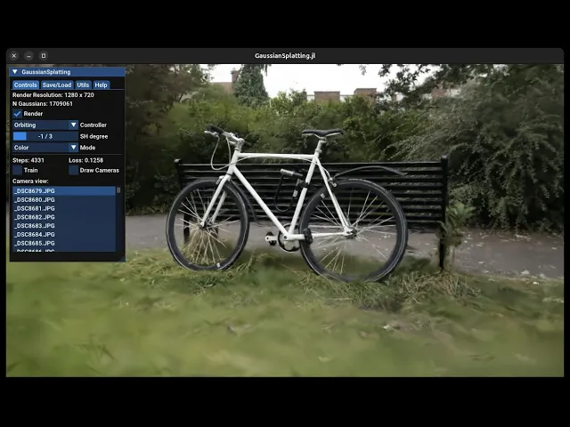
Demo of a GUI application for GaussianSplatting.jl.

At the moment of writing, it supports:

• NVIDIA GPUs & AMD GPUs.

• Windows & Linux.

And features:

• GUI application for training and visualizing gaussians.

• Color / Depth / Uncertainty rendering modes.

• Recording videos given user-defined camera path.

• Saving / loading of trained gaussians.

• Providing generic gaussian rasterization library that can be used by other packages.

To start a GUI application, you start the Julia REPL, import the necessary packages and provide a path to your COLMAP dataset and a scale of images for it:

julia> using CUDA, cuDNN, Flux, GaussianSplatting
julia> GaussianSplatting.gui("<path-to-colmap-dataset>"; scale=4

Use Flux.jl package to switch between different GPU backends (default is CUDA), restart Julia REPL afterwards and launch GUI as described above:

julia> using Flux julia> Flux.gpu_backend!("AMDGPU"

Gaussian Splatting rasterizer is completely implemented in the src/rasterization/ directory of the repository.

To compute gradients of the loss function w.r.t 3D Gaussian parameters we use Automatic-Differentiation (AD) package called Zygote.jl, but since we implement our custom forward and backward GPU kernels it does not know immediately how to use them with the AD system. Therefore, to integrate GPU kernels with it, we use ChainRules.jl.

For the function rasterize , that calls GPU rasterization kernels, you define a rrule for the reverse-mode differentiation which returns the rasterized image (forward pass) and a function (or pullback) that computes the gradients (backward pass):

function ChainRulesCore.rrule(
    ::typeof(rasterize), means_3d, shs, opacities, scales, rotations, ρ = nothing, θ = nothing;
    rast::GaussianRasterizer, camera::Camera, sh_degree::Int,
    background::SVector{3, Float32}, covisibility::Maybe{AbstractVector{Bool}},
)
    image = rasterize(
        means_3d, shs, opacities, scales, rotations, ρ, θ;
        rast, camera, sh_degree, background, covisibility)
    function _rasterize_pullback(∂L∂pixels)
        ∇ = ∇rasterize(
            ∂L∂pixels, means_3d, shs, scales, rotations, ρ, θ,
            rast.gstate.radii; rast, camera, sh_degree, background)
        return (NoTangent(), ∇...)
    end
    return image, _rasterize_pullback
end

And such Chain Rules can be defined for arbitrary functions and GPU kernels providing a very flexible programming model. So in the end, you can write high-level code with the AD system and it will utilize those custom GPU kernels:

backend = CUDABackend()
# 3D Gaussian rasterizer.
rasterizer = GaussianRasterizer(backend, ...)
# 3D Gaussian parameters.
θ = ...
loss, ∇ = Zygote.withgradient(θ...) do μ, rgb, σ, Σ
		# Render 3D Gaussians from a given camera pose.
    rendered_image = rasterizer(μ, σ, Σ, rgb; camera)
    return loss(rendered_image, target_image)
end
# Use computed gradients `∇` to update 3D Gaussians.

Julia Limitations

That said, Julia still has some limitations.

Currently, Julia’s Garbage-Collection (GC) mechanism does not know about GPU memory. So it sees no difference between 1 MiB and 1 GiB allocations, therefore the memory is not freed in time and keeps piling up until there’s no more GPU memory available. At that point we forcibly trigger GC which frees the memory.

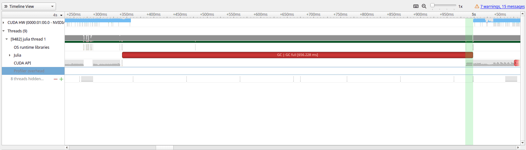
But manually triggering GC is expensive and can take several hundred milliseconds to complete, slowing things down. In the image below you can see that a GC call (red region) takes ~650 ms , but the region where GPU memory is freed is marked with green. This is because calling a GC does garbage collection not only for GPU, but for the whole Julia process.

A solution to this would be to use Reference-Counting GC mechanism that will free GPU arrays immediately as they are no longer used. Some work has been done in that direction, but is still in the early stages.

That said, if your program does not allocate or you manually control the memory you won’t be impacted by this.

Conclusion

Julia language, allowing you to perform both performance-critical low-level as well as high-level programming, offers a solution to the two-language problem and GaussianSplatting.jl is an example of how much simpler the implementation can be, providing smoother development experience.

And with each new Julia version, its GPU capabilities continue to evolve, having fewer and fewer limitations. If you are curious to try Julia, visit Julia website or JuliaGPU for more information.